Learn More about Normal Distribution

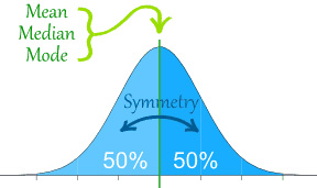
In statistics, the "distribution function" of a random variable is a function that specifies the probability that the variable's observed value will lie in any given region of possible values. The "normal distribution" is the most commonly used distribution in statistics. A variable that is normally distributed has a histogram (or "density function") that is bell-shaped, with only one peak, and is symmetric around the mean. The terms kurtosis ("peakedness" or "heaviness of tails") and skewness (asymmetry around the mean) are often used to describe departures from normality. In a normal distribution, the mean, median, and mode are equal.

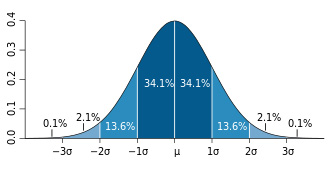
In addition, the normal distribution has few values outside of two standard deviations from the mean.

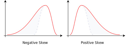
Hardly any nutrient or food group data fit this description. Rather, most are right (positively)-skewed, meaning that the tail on the right side is longer than the one on the left side and the bulk of the values lie to the left of the mean. This is largely due to the fact that there is a very high upper limit on intake but there is a lower limit of zero.

The presence of non-normal distributions can be diagnosed in several ways. Visual inspection of a histogram of the nutrient dietary component is a useful but subjective procedure. Most statistical software packages contain a variety of formal statistical tests for the normal distribution hypothesis, such as the Shapiro-Wilk and Kolmogorov-Smirnov tests.

Because many [glossary term:] parametric statistical procedures assume a normal distribution, it may be necessary to normalize the distribution of skewed dietary data through transformation before analysis. Non-parametric statistical procedures do not have this requirement, and the dietary data can be used without transformation.

When an analysis requires variables to be normally distributed, non-normal dietary data can be transformed to obtain data that better approximate normality. Common transformations used for dietary data include log and power (e.g., square root) transformations. The [glossary term:] Box-Cox transformation, introduced by Box and Cox, is a family of transformations that includes the power and log transformations. To choose the best Box-Cox transformation—the one that best approximates a normal distribution - Box and Cox suggested using the maximum likelihood method. Alternatively, one can choose the transformation that maximizes the Shapiro-Wilk statistic or minimizes the Kolmogorov-Smirnov statistic.

If an analysis involves comparing many dietary variables, it is tempting to transform them all using the same transformation, thereby having them all on the same scale. For example, researchers often use a log transformation across all dietary variables. In some cases, this may be appropriate but the transformed distributions should be examined with regard to non-normality, because all nutrients and food groups are not distributed in a similar way. Although many nutrients are slightly or moderately skewed, some (e.g., vitamin A) may have very skewed distributions.

The Box-Cox transformation parameter also is useful to compare the level of skewness across nutrients. If this parameter varies widely across nutrients, it may be most appropriate to: a) apply the Box-Cox transformation parameter to each nutrient; or b) group nutrients according to their skewness and apply differing Box-Cox power transformations to each group.

Note that it is not always possible to transform a variable to arrive at a distribution that is even approximately normal. Types of variables that cannot be transformed to normality include: discrete variables with only a small number of possible outcomes (e.g., education level, number of times milk is drunk on a given day); variables that have a substantial number of zero values (e.g., usual amount of alcohol consumed (g/day), amount of dark green vegetables consumed on a given day); and variables with multimodal distributions, i.e., those with more than one peak.

For More Information

Box G.E.P. & Cox D.R. (1964) An analysis of transformations. J R Stat Soc B; 26:211-252